JSTML Documentation


JSTML is a intuitive and platform independent program written in Java to analyze SPM measurements done with Omicron Scala software or converted Matrix files.
It is currently the program of choice in the surface science group of Prof. Widdra at the Martin-Luther-University of Halle-Wittenberg and some surface science groups at the
Max Planck Institut for Microstructurephysics
.

Build: 28.01.2010

Download JSTML

wishlist:
- scrolling pane for whole topography window when opening big measurements
- access to single point spectra that were taken at locations outside of topography area
- complete revision of the spectrum map window
- an option that generated a ready-to-submit master thesis chapter

New:
- histogram x-size now scales automatically with window size

fixed Bugs:
- Can't export spectra after deletion of the first spectrum in a spectrum window
- program getting caught in a endless loop when sizing a window very small
- opening of several measurements when browsing topographies too fast with CTRL-Left/Right

Running JSTML

JSTML is programmed in Java. Minimum requirement is Java Runtime Environment 1.5.
You can download the Java Runtime Environment JRE from http://java.sun.com.

To use the OpenGL/DirectX based 3D-Viewer the package Java3D needs to be installed.
You can download Java3D from https://java3d.dev.java.net/

If you are going to use the Measurement Browser with several thousand measurements or 3D-Viewer it is likely that you have to set the maximum memory the JVM can use to a higher value.
It is by default limited to 64 MB. The maximum memory limit can be set with the parameter -XmxAAAM , where AAA is the size in megabytes.
So the command line could look like this:
C:\Program Files\Java\jre1.5.0\bin\java -Xmx512M Stml
Please note that the parameter sets the maximum amount of memory the java application is able to use, not the amount it uses all the time.

You may add a *.par file as command line parameter to open the measurement immediatly.
java -Xmx512M Stml c:\RT\supraconduct\subatomic.par
or
java -Xmx512M -jar jstml.jar c:\RT\supraconduct\subatomic.par


* may change in later versions

Under Linux or MacOS the setup is basically the same. Java, JAI and Java3D might be even available from the package manager, which makes the installation much more comfortable.
Please note that in windows a java update creates a new runtime environment folder, leaving the extension packages in the old runtime environment.
Currently no simple way to circumvent this behaviour is known.
There are two solutions:
- Start JSTML with the java.exe from the old environment.
or Copy the extension DLLs from \bin  and JARs from \lib\ext to the updated runtime environment.
or (worst case) reinstall JAI and Java3D in the updated JRE.
I do not know if this is also a problem in Linux. Though it might also be solved by copying the *.o and *.jar files to the new JRE.
If anyone got a better solution after Java Updates - send me a mail.

Main Window

JSTMl main window The JSTML main window shows the opened measurements and their measurement channels. Another measurement can be picked from the list of files in the folder of the last opened measurement. If you click on a button the corresponding Topography or Spectroscopy-Map window will be opened or brought to the front.

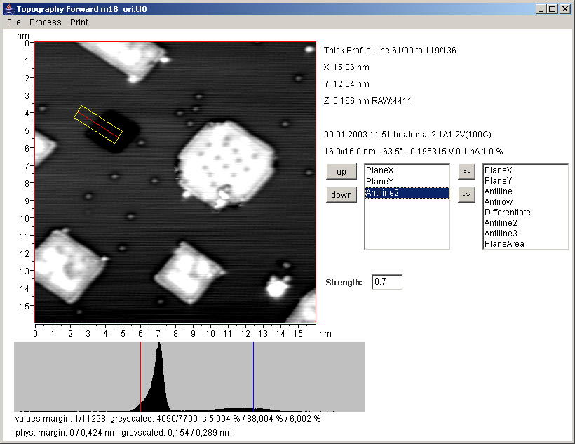
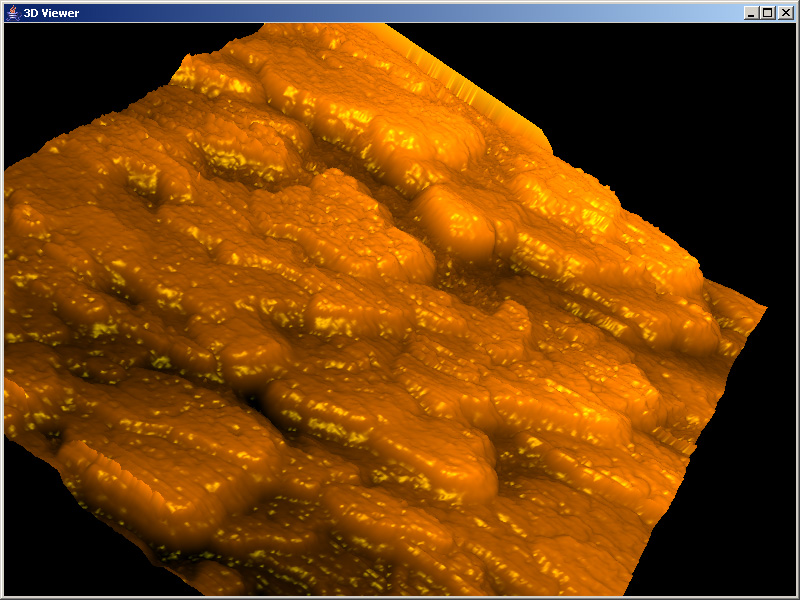
File / Open shows the open dialog for a measurement. All previous measurements will be discarded. The windows for the first topography channel of the measurement is opened.

File / Open Image opens an image like it was a measurement. The data will be considered as 8 bit. On colored images the blue channel is used.

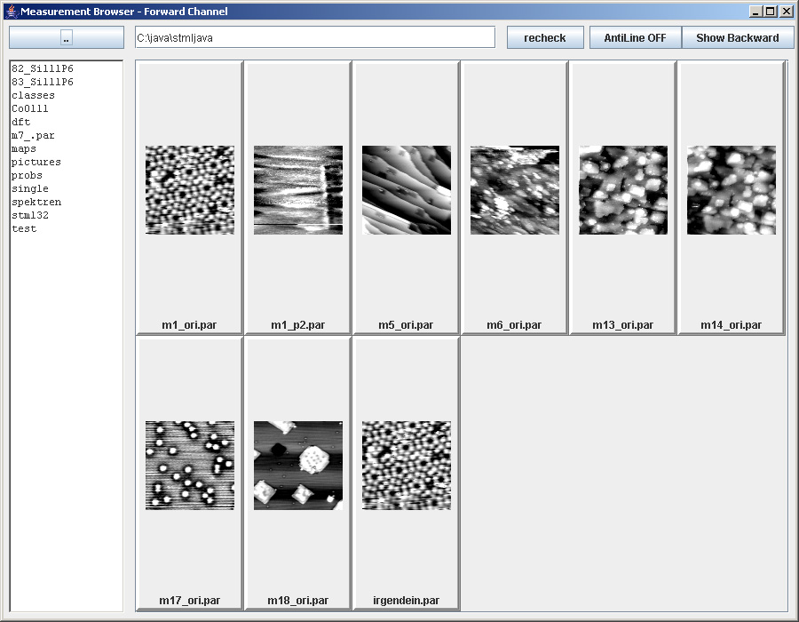
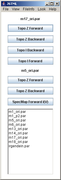
File / Browser opens a measurement browser window. If no *.par file is given as parameter on JSTML startup the browser is opened by default.

View / Options shows the window to enter startup values for different parameters and values used in the program. These are loaded on startup.

FileInfo / ParFile  opens a window that shows all non-specific values from the parameter file. These are all values that are (mainly) not used for Topography and/or Spectroscopy.

Look /  *  changes the Look and Feel of the user interface. The available default skins depend on the installed JRE. You need to reopen a window to let the change take effect.

Help / Online Help opens .this documentation webpage.
Note: the application tries to get the systems default browser. While this works well under Win32 and MacOS, for Linux  by default Firefox is called. Maybe I or someone else finds a better solution here.

Help / Info
short information about the program

Measurement Browser

measurement browser

The Measurment Browser window is a intuitive tool to get a quick overview about many datasets.

Navigation

To navigate through the filesystem you can enter a path in the upper textfield. To get to shares in windows you can also enter a UNC name like \\computer\share\.
If you want to change the drive in windows you have to enter it in the textfield too.
Any valid location pointing to a folder should work.
On the left there is a list with the subfolders of the current path. To change to a subfolder just doubleclick its name.
The button '..' goes one folder up.
Pressing  ENTER in the textfield rereads the current folder and all thumbnails.

Measurement Preview

If there are measurements in the current folder thumbnails are generated and displayed in the scrollpane. The thumbnail size can be set in the options dialog.
Some default filters are applied to the datasets to give optimum viewability of the data. These are:
The thumbnails are sorted ascending by the Omicron naming convention: mXXX_*.par where XXX is a number. After them the files are added that doesn't fit in this convention.
Moving the mouse over a thumbnail gives a tooltip with filename, size and gap voltage information of the measurement.
The button recheck rereads the current folder and adds new files to the end of the thumbnails
The button AntiLine OFF/ON de/activates the AntiLine filter. Pressing this button results in a reread of the current folder.
After the browser has read through a folder of measurements, all available topography channels will be added to the Show menu.
Then you can choose another channel and thumbnails for that channel will be generated. This results in a reread of the current folder.
Be aware that f.e. the second topography channel on different measurements can be also different, even not available for each measurement in the folder.
If there is no data file for the specified chosen channel the image label will be greyed out.

Clicking left on a thumbnail discards all other opened measurements and opens the clicked one.
Clicking right on a thumbail adds the measurement to the already opened ones.
The topography windows of the first topography channel of each measurement will be opened or brought to front if already opened.
Holding CTRL while moving the mouse over a measurement brings up a list with some additional information.

Topography Window

Topography Window

The topography window displays the topography as greyscaled image surrounded by axis. The point 0,0 is located at the upper left as used in older Scala versions.
The image is scaled depending on the size of the window.
On the top right a textline gives the status of the currently selected tool. Below this the data of the current X,Y,Z position is monitored as the mouse is moved over the image.
Then two lines with the most important measurement informations follow.

Filters

The two lists represent the active (left) and available (right) filters. The active filters in the left list are applied in the order they appear in the list.
With the buttons '<-' and '->' filters can be added to or removed from the list of active filters. By choosing a filter in the left list and pressing the button
'up' or 'down' the order can be changed. If an active filter is selected the corresponding panel with its properties is displayed below.
The default filters applied on opening a topography window can be set in the options dialog.

Histogram

The histogram shows the distribution of the values of the topography. The red line marks the lower cap and the blue line the higher cap of the grey levels.
All points with lower values than marked by the red line are black.
All points with higher values than marked by the blue line are white.
The grey levels are distributed linear in between.
By default the histogram border part defined in the options dialog gives the position of the red and blue line after filters are applied.
The value is by default 0.06 that means that 6 %  of the histogram volume on the low end and on the high end will be made black or white.
This is to exclude rare measurement distortion points to destroy the contrast of the overall image.

However the lines defining the caps can be set with the mouse. A left click in the histogram area sets the position of the red line (lower cap), a right click sets the position
of the blue line (higher cap). The contrast is adjusted immediatly.
Notice that you cannot set the blue line below the red line and vice versa. (For reversing grey levels you can use a colormap.)

The text below the histogram gives the raw values of the whole dataset and the ones displayed in grey levels. The percent values give the partial areas of the image that correspond to the
black / greyscaled / white areas. The sum of all percent values gives 100% - the whole image. This can be used to measure coverages.
Example: If you got islands on a plane substrate you set the contrast that the islands are greyscaled and read the percent value in the middle.

The second text line gives the values of the line above in physical units.

Menu

File / Next File (Ctrl+right)  discards this measurement and replaces it with the next one in the folder of this measurement. The order used is the same as the measurement browser uses.
File / Previous File (Ctrl+left)  discards this measurement and replaces it with the previous one in the folder of this measurement. The order used is the same as the measurement browser uses.
Both functions will wrap around at the first/last file.
File / Load Colormap  opens a filedialog to load a *.png colormap. (colormap format) The colormap is linear distributed instead of the greylevels.
File / Colormap off  switches the application of a colormap off - back to greylevels.
File / Save Image  (Ctrl+S) opens the save image dialog and saves the image as displayed on the screen in the given color depth.
File / Save Image with Infos  (Ctrl+V) saves a image in PNG format. The image content is identical as it would have been printed. The PNG format is RGB with 8 bits per channel and an alpha-channel. So the background is transparent.
This is very useful if you want to add it to a presentation (like a poster) with custom background.
File / Show 3D View (Ctrl+3) shows the image as set by the histogram caps in the 3D Viewer
File / Play as sound plays the data as 16bit soundsample with 8000 data points per seconds.

Process / Contrast Area (Ctrl+A) Choosing this, you can drag a rectangle on the image (green line border) that marks an area for that the maximum and minimum value is determined.
Based on these values the contrast of the whole image is set that the greylevels are distributed over this area. The red and blue histogram line is set accordingly.
This can also be used to mask islands or planes.
Process / Subtract Plane Area You can drag a rectangle on the image that marks an area for that the minimum value is determined. The lower cap - red line of the histogram is set to this value.
Notice that this way the red line can be set higher than the high cap - blue line. This will result in a black / white image with the red line as treshold.
Process / Profile Line  (Ctrl+L) By choosing this you can draw a line on the image. Left click to set the start point then move the mouse and left click again to set the end point. By setting the end point the datapoints the line touches are taken in a XY-spectrum window. Note that the X-axis corresponds to the path along the drawn line and that the X-values are not equidistant.
Process / Thick Profile Line (Ctrl+T) A tool to draw a thick profile line to average over more data points. Opens a dialog requesting the thickness of the profile line. The drawing of the line works the same way as for the Profile Line. The corresponding thick line is shown as yellow rectangle. As of writing this documentation the subsampling for averaging is 1/5 th pixels in both directions.
After setting the end point the name for a spectrum window is requested. As long as this tool is active and the thick profile line is drawn over the image you can move to a point on the image and
right click. This rotates the set Thick Profile Line by 90 degress CCW and requests a spectrum window name.
This can be used to draw the profile line exactly along a given feature and then average (also exactly) perpendicular to it.
Process / Zoom Area (Ctrl+Z) You can drag a rectangle on the image and the topography will zoom in this area.
Process / Zoom Dialog Opens a dialog where you can enter the zoom area in physical units.
Process / Unzoom (Ctrl+U) restores the size of the original measurement
Process / Get Drift (Ctrl+D) if activated you can set a start point with left click and a end point with right click on the image. All open topography windows show the physical correct scaled representation of the set vector.
You can set the points in every topography window. The distance and angle is show in the tooltext. If the start and/or end point doesn't fit in a specific topography image the line is not drawn.
Example: You got topography1 and a drifted topography2 of the same area. You set the start point at some characteristic feature in topography1 and switch to topography2 and set there the end point at the same feature. The tooltext shows the distance.
Process / FFT experimental does a FFT transformation of the data and shows it in the FFT-window. This can be used as 'local LEED'.
Alot more things are planned here to be implemented (transformation back, step functions)
Process / INT Zoom only (Ctrl+I)  if activated the image is scaled in the window only in multiples of whole numbers. If you don't scale the image in the window in multiples of whole numbers you might experience artifacts from scaling that are not present in the data - you have been warned.
Process / Show Limits (Ctrl+H) if activated shows the areas where histogram caps apply. Red for points with a value lower than the red line marks and blue for a value higher than the blue line marks.

Spectras / Channel X if there were single point spectroscopy measured the active spectroscopy channels get listed here. On activation small red squares with the number of the spectrum are displayed above the image. By moving the mouse close to one you choose it (it gets yellow) and by clicking it asks for the name of the spectrum window the single point spectrum should be put into.
You can also mark an area holding down the left mouse button to choose several spectra that will be put in a window.
A small spectrum preview will be shown of the closest spectrum to the mouse cursor.
Note: If the location the spectra was taken (x,y) is at the wrong spot please drop me a mail.

Print / Print Graphics (Ctrl+P) opens the systems printer dialog and then print layout dialog.

SpectrumMap Window

spectrummap window

The spectrum map window displays a mapped spectroscopy dataset. An image represents the map at a certain voltage for I(V) (a certain Z for I(Z) and so on...).
The histogram has identical functionality like in the topography window.
On the right side the number of the point in the spectra the map image is made from is displayed in the textfield. It can also be set by the user.
The corresponding physical value is displayed below. The maps can also be switched through by clicking the buttons '<' respectivly '>'.

If you click left in the image the spectrum at this point will be taken to a spectrum window.

Menu

File / Save Image opens the save image dialog and saves the image as displayed on the screen in the given color depth.

Selection / Show Selection on activation the selection panel appears on the right. With this panel you can select multiple spectra that is marked by a small red cross.
The panel gives three modes of selection:
Pressing Takeover adds all selected spectra to a spectrum window.
Example: You choose in a I(V) map a voltage where the image shows a high contrast between characteristic features. You select 'local by tolerance' and draw the line over one feature, selecting only spectra that show this specific contrast at this particular voltage.
Selection / Deselect All deselects all spectra points.
Show in Topo shows the location of the marked spectra in the topography window. It does an automatically update if you use the tolerance selection modes, for single point selection you have to update the topography manually by activating Show in Topo. The marked points in topography do not count towards overlay but to image.

Print / Print Graphics opens the systems printer dialog and then print layout dialog.

Spectrum Window

Spectrum Window

A spectrum window shows one or more spectra. By moving or dragging the mouse you can measure distances in X and Y.
The currently chosen spectrum is black, the others are red.

Menu

Spectras / Spectrum X  selects the current spectrum. Notice: if there are too many spectra added to the window this menu will be disabled, but you can still switch through with ctrl+left and ctrl+right.

Range / Set Range  opens a dialog to set the values for start and end value of the axis.
Range / Autorange  sets the axis to the minimum and maximum values of the spectra. So all data is visible in the diagram area.

Process / Remove Spectrum  removes the currently selected spectrum from the spectrum window
Process / Copy to Frame  copies the currently selected spectrum to another spectrum frame.
Process / Average All   generates a spectrum that is averaged over all spectra in the spectrum window.
Process / dY / dX  differentiates the selected spectrum. Since the numerical differentiated spectrum would have a point less for compatibility an additional point is added at the end of the spectrum.
Note: This detail might me outdated and removed in later versions
Note: The physical units might have a untypical naming like dI / dV instead of dI / dU. The program takes the naming from the parameter file.
Process / Export Spectrum  opens a file dialog to export the selected spectrum as plain text. The format of the file is:
View / Next Spectrum (ctrl+right) selects the next spectrum
View / Previous Spectrum (ctrl+left) selects the previous spectrum
View / Edit Legend opens a dialog where you can edit the Name of the Frame, the physical unit of the X and Y axis and the name shown in the spectrum.

Print / Print Graphics opens the systems printer dialog and then print layout dialog.

3D Viewer

3d Viewer

The 3D-Viewer displays the topography data as a 3D representation. This is mainly useful for presentation issues.
The topography is taken as set with the histogram, so greylevels correspond to heights. Typically it is useful to set the histogram caps a little broader to avoid caps in the 3D representation.
Before the 3D window appears a settings dialog appear.
There you set the color of the surface or select a colormap. The metallic look adds a specular light and some shinyness to the surface. Without shinyness the surface will appear matt.
The topography data will be scaled by the values given by XY Zoom and Z Zoom.
Pressing Show generated the 3D data and puts the 3D surface into a window.
Be aware that probably several million triangles are calculated and moving this to the driver may take a moment.
If you encounter a java.OutOfMemory.Exception try to give the JVM more memory.
Any hardware 3D acceleration is recommended.

The mouse behaviour keys for the 3D window are as follows:
The following additional keys are defined:
Please note that Java3D is still a Beta.

Option Window

The option window is splitted in several panels. You can switch between by pressing '<' or ">' respectivly.
On 'Save' a file called stml.ini will be written to the folder stmljava in the users home folder.
The option file is in text format, though I do not recommend to edit it by hand. If there are problems with the options,
delete the file. On JSTML startup a default configuration will be written.

Directories

Browser Directory  the folder the measurement browser opens first.
Images Directory the default folder for saving images filedialog
Export Directory the default folder for export spectrum filedialog
Export Seperator the seperator used for plain text exportet spectra data
Use Multithreading enables multithreading where implemented. Currently only the Measurement Browser supports this for thumbnail generation. This is taken over at once.
Threads maximum number of  concurrently running threads. This is taken over on reopening a Browser window.
Hint: The console displays the time used to generate the thumbnails, so might tweak it a bit for your specific system.

Histogram options

Histogram borders  the fraction of histogram volume capped by default. default value is 0.06, corresponding to 6 %.
Histogram size Size of the histogram image

Topography Options

Plane  adds PlaneX and PlaneY by default to the active filter list in a topography window
Antiline2  adds Antiline2 by default to the active filter list in a topography window
Differentiate adds Differentiate by default to the active filter list in a topography window
Differentiate Weights  sets the default weights for the differentiate filter

Print Options

not used anymore, will be removed in one of the next versions.

View Options

Spectrum Window size  size of any new spectrum window
Browser thumbnail size size of a thumbnail generated in the measurement browser
More greylevels adds more greylevels than the usual possible 256 by varying the RGB values by a maximum of +-2. Based on the NTSC color vs brightness weighting that applies to the current displays and the eyes sensitivity  varying the Red Green and Blue component around the main grey path with R=G=B makes it possible to give a pixel a brightness intensity thats in between.
The weighting is I = 0.3 * R + 0.59 * G + 0.11 * B.
Based on this the following table is applied:
  double inttab[]={0,0.11,0.18,0.19,0.22,0.29,0.3,0.4,0.41,0.48,0.52,0.59,0.6,0.7,0.71,0.78,0.81,0.82,0.89};
  int      rtab[]={0,0   ,-1  ,1   ,0   ,-1  ,1  ,-1 ,1   ,0   ,1   ,0   ,2  ,0  ,2   ,1   ,0   ,2   ,1   };
  int      gtab[]={0,0   ,1   ,0   ,0   ,1   ,0  ,1  ,0   ,1   ,0   ,1   ,0  ,1  ,0   ,1   ,1   ,0   ,1   };
  int      btab[]={0,1   ,-1  ,-1  ,2   ,0   ,0  ,1  ,1   ,-1  ,2   ,0   ,0  ,1  ,1   ,-1  ,2   ,2   ,0   };
The inttab array represents the resulting intensity offset from the R,G,B variation. The slight coloring of the pixel is not visible with the eye.
Interpolate Thick Profile Line triangulates between data points and does this way a linear interpolation of the intermediate grid points when drawing a Thick Profile Line
Integer zoom only zooms only in integer steps to prevent artifacts in view.

Filters

Filters are routines that change the data. It is to the user to use the filters available in the right manner. This needs a basic understanding what each filter does.
For example it doesn't make sense to measure heights in a differentiated topography.

PlaneX

Calculates the plane below the dataset in X-direction and subtracts it. Internal a linear regression of the averaged rows is calculated. Thsi filter has no property panel.

PlaneY

Same functionality as PlaneX just for Y-direction.

Antiline

Classic offset subtraction line by line. For each line the average is calculated and the difference determined to the averaged height of the whole image. This offset is subtracted from the line.
This filter has problems with islands on planes. Due to the averaging the underlying plane will be moved to lower values. This typically gives stripes in the data.

Antirow

Same functionality as Antiline just for the rows (Y-direction)

Differentiate

Applies a local differentation to the data. The value of a point depends on a weighting of its neighbours. A point has four direct neighbours and itself, that gives five weight factors.
The weighted point is calculated by the sum of (weight * point_value) of all five points. 
The property panel has textfields for the weights, the textfields are layouted like the neighbour points. The startup values can be set in the options dialog.
This filter gives a high contrast on small topographic changes, though the values can't be treated as real heights anymore.
Typically only the X-direction is differentiated because of the strong correlation between these values.
Example: To get the first derivation in X enter -1 , 0 , 1. To get the second derivation -5, 10 , -5.

Antiline2

This filter is more complex than the classic Antiline and has certain advantages. The main advantage is that it keeps planes.
Basically it calculates the offset to the previous line considering for this only special points (not all).
At first a histogram of the difference to the values to the previous line is made. Then the smallest area including the histogram volume given by the property panel parameter is searched.
All points in this area are taken into account when calculating the offset to the previous line.
Physically this means that the points where both lines have most similar corrugation behaviour will be taken for offset calculation.
The property panel parameter is a value between 0 and 1 and gives the part of the histogram volume taken into account.
This is directly related to the fraction of points of a line taken for offset calculation. A value of 1 makes this filter working (nearly) the same way as the classic antiline.
Higher values make the offset calculation more precise at the cost taking more points into account that have a not similar corrugation like the previous line.
As a rule of thumb - the sharper the peaks in the histogram of the whole image, the better the offset correction worked.

Antiline3

Just a working name for a filter with a not so local behaviour (and the related problems) as antiline2. Currently it shows the points taken into account for calculation for antiline2 as white.

PlaneArea

With this filter you can mark points that are used to subtract the underlying plane from the whole image. When this filter is selected in the active filter list you can drag a rectangle on the image
to mark areas that are show as green points. If you use the right button to drag the chosen area will be unmarked. If you press the Clear button in the property panel the whole image will be unmarked.
Pressing Takeover applies the marked points for plane calculation.
This can be used to plane a topography depending on a specific plane in the image.

PlaneArea2

This Filter is a combination of Antiline2 and PlaneArea. With a Antiline2 filter a percentage of points is excluded. These points have unusual strong local 'height' variation. So only the points on a flat surface are taken into account for calculation of the plane. This has the advantage that you can mark a rectangular area over a measurement area with local distortions. With the right set AntiLine2 percentage the distorted points will be excluded for the plane calculation. If you check 'Show excluded points' the excluded points will be set to maximum histogram value and this way they are shown 'white'. Do not use this view for further data analysis - always uncheck 'Show excluded points' again !

Save Image Dialog

If you save an image this dialog appears and let you choose the format of the image. For visual representation a 8 bit format is suitable. Please keep in mind that JPEG is not a lossless compression. Any application that has image processing capabilities should be able to open this.
For further data analysis 16 bit should be enough, before saving you can check the raw values below the histogram if the data fits in 16 bit. Good applications can handle this format.
For enthusiasts 32 bit TIFF is a must, but be aware that only a few applications can read this format.

Print Layout Dialog

This dialog appears after the systems printer dialog and  JSTML got the necessary information. You can choose where the graphics should be printed on the page.
With factor Shrink you can scale the graphics even smaller - a value of 2 corresponds to the half size.
Currently you have to reinsert the page into the printer again to print different graphics to different locations.
(JSTML does not collect print output)

Colormap Format

A colormap is a *.png image. The first horizontal line of the image is taken as the colormap. So the number of horizontal pixels is the number of colors in the map.
The color at this position is given by the color of the pixel. All following lines (y > 1) are ignored.
With a colormap greater than 256 more visible steps can be achieved.

Known Bugs

I would like to say that there are no bugs but that would be a lie ;)
So here we go:

Credits

Program and this documentation by Michael Huth